License is MIT: see https://github.com/JuliaFEM/JuliaFEM.jl/blob/master/LICENSE.md

2D Hertz contact problem

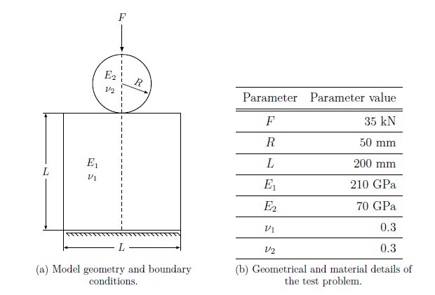In the example, a cylinder is pressed agains block with a force of 35 kN. A similar example can be found from NAFEMS report FENET D3613 (advanced finite element contact benchmarks). Solution for maximum pressure $p_0$ and contact radius $a$ is

\[ p_{0} = \sqrt{\frac{FE}{2\pi R}}, \\ a = \sqrt{\frac{8FR}{\pi E}},\]

where

\[ E = \frac{2E_{1}E_{2}}{E_{2}\left(1-\nu_{1}^{2}\right)+E_{1}\left(1-\nu_{2}^{2}\right)}.\]

Substituting values, one gets accurate solution to be $p_0 = 3585 \;\mathrm{MPa}$ and $a = 6.21 \;\mathrm{mm}$.

using JuliaFEM, LinearAlgebra

Simulation starts by reading the mesh. Model is constructed and meshed using SALOME, thus mesh format is .med. Mesh type is quite simple structure, containing things like mesh.nodes, mesh.elements and so on. Keep on mind, that Mesh contains only standard Julia types and we think it as a structure helping us to construct elements needed in simulation. In principle, we don't need to use Mesh in simulation anyway if we figure some other way to define the geometry for elements.

datadir = abspath(joinpath(pathof(JuliaFEM), "..", "..", "examples", "2d_hertz_contact"))
meshfile = joinpath(datadir, "hertz_2d_full.med")
mesh = aster_read_mesh(meshfile)
for (elset_name, element_ids) in mesh.element_sets
    nel = length(element_ids)
    println("Element set $elset_name contains $nel elements.")
end
for (nset_name, node_ids) in mesh.node_sets
    nno = length(node_ids)
    println("Node set $nset_name contains $nno nodes.")
end
nnodes = length(mesh.nodes)
println("Total number of nodes in mesh: $nnodes")
nelements = length(mesh.elements)
println("Total number of elements in mesh: $nelements")

[ Info: Mesh parsed from Code Aster file /home/travis/build/JuliaFEM/JuliaFEM.jl/examples/2d_hertz_contact/hertz_2d_full.med.
[ Info: Mesh contains 275 nodes and 557 elements.
[ Info: Element set FIXED contains 10 elements (10 x Seg2).
[ Info: Element set OTHER contains 63 elements (63 x Seg2).
[ Info: Element set BLOCK_TO_CYLINDER contains 6 elements (6 x Seg2).
[ Info: Element set CYLINDER_TO_BLOCK contains 6 elements (6 x Seg2).
[ Info: Element set SYM23 contains 11 elements (11 x Seg2).
[ Info: Element set CYLINDER contains 133 elements (133 x Tri3).
[ Info: Element set BLOCK contains 328 elements (328 x Tri3).
Element set FIXED contains 10 elements.
Element set OTHER contains 63 elements.
Element set BLOCK_TO_CYLINDER contains 6 elements.
Element set CYLINDER_TO_BLOCK contains 6 elements.
Element set SYM23 contains 11 elements.
Element set CYLINDER contains 133 elements.
Element set BLOCK contains 328 elements.
Node set CYLINDER_LOAD contains 1 nodes.
Node set OTHER contains 270 nodes.
Node set CYLINDER_CONTACT_POINT contains 1 nodes.
Node set CYLINDER_RIGHT contains 1 nodes.
Node set BLOCK_CONTACT_POINT contains 1 nodes.
Node set CYLINDER_LEFT contains 1 nodes.
Total number of nodes in mesh: 275
Total number of elements in mesh: 557

Next, define two bodies. Technically, we could have only one problem and add elements from both bodies to the same problem, but defining two different problems is recommended for clarity. Plain strain assumption is used. To make clear what is happening here: we first create a set of elements (elements are in vector called upper_elements), then we define new problem which type is Elasticity, give it some meaningful name (this time cylinder), and last value 2 means that problems does have two degrees of freedom per node.

upper_elements = create_elements(mesh, "CYLINDER")
update!(upper_elements, "youngs modulus", 70.0e3)
update!(upper_elements, "poissons ratio", 0.3)
upper = Problem(Elasticity, "cylinder", 2)
upper.properties.formulation = :plane_strain
add_elements!(upper, upper_elements)
lower_elements = create_elements(mesh, "BLOCK")
update!(lower_elements, "youngs modulus", 210.0e3)
update!(lower_elements, "poissons ratio", 0.3)
lower = Problem(Elasticity, "block", 2)
lower.properties.formulation = :plane_strain
add_elements!(lower, lower_elements)

[ Info: Created 133 elements (133 x Tri3) from element set: CYLINDER.
[ Info: Updating field `youngs modulus` => 70000.0 for 133 elements.
[ Info: Updating field `poissons ratio` => 0.3 for 133 elements.
[ Info: Creating a new problem of type Elasticity, having name `cylinder` and dimension 2 dofs/node.
[ Info: Adding 133 elements to problem `cylinder`
[ Info: Created 328 elements (328 x Tri3) from element set: BLOCK.
[ Info: Updating field `youngs modulus` => 210000.0 for 328 elements.
[ Info: Updating field `poissons ratio` => 0.3 for 328 elements.
[ Info: Creating a new problem of type Elasticity, having name `block` and dimension 2 dofs/node.
[ Info: Adding 328 elements to problem `block`

Next we define some boundary conditions: creating "boundary" problems goes in the same way than defining "field" problems, the only difference is that we add extra argument giving what field are we tring to fix. This time, we have 2 dofs / node and we fix displacement in direction 2.

bc_fixed_elements = create_elements(mesh, "FIXED")
update!(bc_fixed_elements, "displacement 2", 0.0)
bc_fixed = Problem(Dirichlet, "fixed", 2, "displacement")
add_elements!(bc_fixed, bc_fixed_elements)

[ Info: Created 10 elements (10 x Seg2) from element set: FIXED.
[ Info: Updating field `displacement 2` => 0.0 for 10 elements.
[ Info: Creating a new boundary problem of type Dirichlet, having name `fixed` and dimension 2 dofs/node. This boundary problems fixes field `displacement`.
[ Info: Adding 10 elements to problem `fixed`

Defining symmetry boundary condition goes with the same idea

bc_sym_23_elements = create_elements(mesh, "SYM23")
update!(bc_sym_23_elements, "displacement 1", 0.0)
bc_sym_23 = Problem(Dirichlet, "symmetry line 23", 2, "displacement")
add_elements!(bc_sym_23, bc_sym_23_elements)

[ Info: Created 11 elements (11 x Seg2) from element set: SYM23.
[ Info: Updating field `displacement 1` => 0.0 for 11 elements.
[ Info: Creating a new boundary problem of type Dirichlet, having name `symmetry line 23` and dimension 2 dofs/node. This boundary problems fixes field `displacement`.
[ Info: Adding 11 elements to problem `symmetry line 23`

Next we define point load. To define that, we first need to find some node near the top of cylinder, using function find_nearest_node. Then we create a new problem, again of type Elasticity. Like told already, we don't need to use Mesh if we have some other procedure to define the geometry of the element (and it's connectivity, of course). So we can directly create an element of type Poi1, meaning 1-node point element, update it's geometry and apply 35.0e3 kN load in negative y-direction:

nid = find_nearest_node(mesh, [0.0, 100.0])
load = Problem(Elasticity, "point load", 2)
load.properties.formulation = :plane_strain
load.elements = [Element(Poi1, [nid])]
update!(load.elements, "geometry", mesh.nodes)
update!(load.elements, "displacement traction force 2", -35.0e3)

[ Info: Creating a new problem of type Elasticity, having name `point load` and dimension 2 dofs/node.
[ Info: Updating field `geometry` for 1 elements.
[ Info: Updating field `displacement traction force 2` => -35000.0 for 1 elements.

Next, we define another boudary problem, this time the type of problem is Contact2D, which is a mortar contact formulation for two dimensions. Elements are added using add_slave_elements! and add_master_elements!. Problems, in general, can have some properties defined, like the formulation in Elasticity (we also have :plane_stress). For contact, we need to swap normal direction for meshes created by SALOME because in Code Aster, element orientation is defined opposite to what is used in ABAQUS, and in JuliaFEM in general we follow the same conventions what are used in ABAQUS.

contact = Problem(Contact2D, "contact", 2, "displacement")
contact.properties.rotate_normals = true
contact_slave_elements = create_elements(mesh, "BLOCK_TO_CYLINDER")
contact_master_elements = create_elements(mesh, "CYLINDER_TO_BLOCK")
add_master_elements!(contact, contact_master_elements)
add_slave_elements!(contact, contact_slave_elements)

[ Info: Creating a new boundary problem of type Contact2D, having name `contact` and dimension 2 dofs/node. This boundary problems fixes field `displacement`.
[ Info: Created 6 elements (6 x Seg2) from element set: BLOCK_TO_CYLINDER.
[ Info: Created 6 elements (6 x Seg2) from element set: CYLINDER_TO_BLOCK.

After all problems are defined, we define some Analysis, which can be e.g. static analysis, dynamic analysis, modal analysis, linear perturbation analysis and so on. Here, the analysis type is Nonlinear, which is nonlinear quasistatic analysis. In the same manner as we do add_elements! to add elements to Problem, we use add_problems! to add problems to analysis. Because we are not restricted to some particular input and output formats, we "connect" a ResultsWriter to our analysis, this time we want to visualize results using ParaView, thus we write our results to Xdmf format, which uses well defined standards XML and HDF to store model data.

analysis = Analysis(Nonlinear)
add_problems!(analysis, upper, lower, bc_fixed, bc_sym_23, load, contact)
xdmf = Xdmf("2d_hertz_results"; overwrite=true)
add_results_writer!(analysis, xdmf)

[ Info: Creating a new analysis of type Nonlinear with name `Nonlinear Analysis`.
[ Info: Adding problem `cylinder` to analysis `Nonlinear Analysis`.
[ Info: Adding problem `block` to analysis `Nonlinear Analysis`.
[ Info: Adding problem `fixed` to analysis `Nonlinear Analysis`.
[ Info: Adding problem `symmetry line 23` to analysis `Nonlinear Analysis`.
[ Info: Adding problem `point load` to analysis `Nonlinear Analysis`.
[ Info: Adding problem `contact` to analysis `Nonlinear Analysis`.

In last part, we run the analysis.

run!(analysis)
close(xdmf)

[ Info: --------------------------------------------------------------------------------
[ Info: Starting nonlinear iteration #1
[ Info: Increment time t=0.0
[ Info: --------------------------------------------------------------------------------
[ Info: Updating field `normal` for 6 elements.
[ Info: Updating field `tangent` for 6 elements.
[ Info: First contact iteration, initial contact state = AUTO
[ Info: Average weighted gap = 8.274499442961543, std gap = 6.196825080185221, automatically determined contact state = UNKNOWN
[ Info: # | A | I | St | Sl | gap | pres | comp
[ Info: 122 | 0 | 1 |  0 |  0 | 14.938 | 0.0 | -14.938
[ Info: 133 | 0 | 1 |  0 |  0 | 11.566 | 0.0 | -11.566
[ Info: 134 | 0 | 1 |  0 |  0 | 2.457 | 0.0 | -2.457
[ Info: 135 | 0 | 1 |  0 |  0 | 0.0 | 0.0 | -0.0
[ Info: 137 | 0 | 1 |  0 |  0 | 13.236 | 0.0 | -13.236
[ Info: 144 | 0 | 1 |  0 |  0 | 2.968 | 0.0 | -2.968
[ Info: 145 | 0 | 1 |  0 |  0 | 12.757 | 0.0 | -12.757
[ Info: Solving linear system.
[ Info: Solved linear system in 0.11 seconds using solver 1. Solution norms (||u||, ||la||): (2.593394620027438e15, 31677.866594832423).
[ Info:
[ Info: --------------------------------------------------------------------------------
[ Info: Starting nonlinear iteration #2
[ Info: Increment time t=0.0
[ Info: --------------------------------------------------------------------------------
[ Info: Updating field `normal` for 6 elements.
[ Info: Updating field `tangent` for 6 elements.
[ Info: # | A | I | St | Sl | gap | pres | comp
[ Info: 122 | 1 | 0 |  0 |  1 | -1.0161082927284144e15 | 0.0 | 1.0161082927284144e15
[ Info: 133 | 1 | 0 |  0 |  1 | -1.962185119553583e15 | 0.0 | 1.962185119553583e15
[ Info: 134 | 1 | 0 |  0 |  1 | -1.8135172199303708e15 | 0.0 | 1.8135172199303708e15
[ Info: 135 | 1 | 0 |  0 |  1 | -1.796453121243904e15 | 0.0 | 1.796453121243904e15
[ Info: 137 | 1 | 0 |  0 |  1 | -8.972056937770969e14 | 0.0 | 8.972056937770969e14
[ Info: 144 | 1 | 0 |  0 |  1 | -1.932419818881688e15 | 0.0 | 1.932419818881688e15
[ Info: 145 | 1 | 0 |  0 |  1 | -1.900612784520093e15 | 0.0 | 1.900612784520093e15
[ Info: Solving linear system.
[ Info: Solved linear system in 0.72 seconds using solver 3. Solution norms (||u||, ||la||): (2.5933946200274195e15, 82357.76148154144).
[ Info:
[ Info: --------------------------------------------------------------------------------
[ Info: Starting nonlinear iteration #3
[ Info: Increment time t=0.0
[ Info: --------------------------------------------------------------------------------
[ Info: Updating field `normal` for 6 elements.
[ Info: Updating field `tangent` for 6 elements.
[ Info: # | A | I | St | Sl | gap | pres | comp
[ Info: 122 | 0 | 1 |  0 |  0 | -0.053 | -27236.723 | -27236.67
[ Info: 133 | 1 | 0 |  0 |  1 | -0.282 | 1641.563 | 1641.845
[ Info: 134 | 1 | 0 |  0 |  1 | -0.045 | 5184.482 | 5184.527
[ Info: 135 | 1 | 0 |  0 |  1 | -0.132 | 6554.88 | 6555.012
[ Info: 137 | 0 | 1 |  0 |  0 | 0.056 | -22934.526 | -22934.582
[ Info: 144 | 1 | 0 |  0 |  1 | 0.018 | 5026.36 | 5026.342
[ Info: 145 | 1 | 0 |  0 |  1 | 0.282 | 2387.682 | 2387.4
[ Info: Solving linear system.
[ Info: Solved linear system in 0.01 seconds using solver 3. Solution norms (||u||, ||la||): (10.514336619389132, 14737.61979295678).
[ Info:
[ Info: --------------------------------------------------------------------------------
[ Info: Starting nonlinear iteration #4
[ Info: Increment time t=0.0
[ Info: --------------------------------------------------------------------------------
[ Info: Updating field `normal` for 6 elements.
[ Info: Updating field `tangent` for 6 elements.
[ Info: # | A | I | St | Sl | gap | pres | comp
[ Info: 122 | 0 | 1 |  0 |  0 | 9.339 | 0.0 | -9.339
[ Info: 133 | 0 | 1 |  0 |  0 | 0.0 | -3654.818 | -3654.818
[ Info: 134 | 1 | 0 |  0 |  1 | -0.0 | 4213.666 | 4213.666
[ Info: 135 | 1 | 0 |  0 |  1 | 0.0 | 5593.937 | 5593.937
[ Info: 137 | 0 | 1 |  0 |  0 | 7.905 | 0.0 | -7.905
[ Info: 144 | 1 | 0 |  0 |  1 | -0.0 | 3889.884 | 3889.884
[ Info: 145 | 0 | 1 |  0 |  0 | -0.0 | -4278.92 | -4278.92
[ Info: Solving linear system.
[ Info: Solved linear system in 0.01 seconds using solver 3. Solution norms (||u||, ||la||): (5.554788342076323, 11615.586412659957).
[ Info:
[ Info: --------------------------------------------------------------------------------
[ Info: Starting nonlinear iteration #5
[ Info: Increment time t=0.0
[ Info: --------------------------------------------------------------------------------
[ Info: Updating field `normal` for 6 elements.
[ Info: Updating field `tangent` for 6 elements.
[ Info: # | A | I | St | Sl | gap | pres | comp
[ Info: 122 | 0 | 1 |  0 |  0 | 11.786 | 0.0 | -11.786
[ Info: 133 | 0 | 1 |  0 |  0 | 6.698 | 0.0 | -6.698
[ Info: 134 | 1 | 0 |  0 |  1 | 0.0 | 821.411 | 821.411
[ Info: 135 | 1 | 0 |  0 |  1 | -0.0 | 4056.018 | 4056.018
[ Info: 137 | 0 | 1 |  0 |  0 | 10.427 | 0.0 | -10.427
[ Info: 144 | 1 | 0 |  0 |  1 | -0.0 | 583.517 | 583.517
[ Info: 145 | 0 | 1 |  0 |  0 | 7.788 | 0.0 | -7.788
[ Info: Solving linear system.
[ Info: Solved linear system in 0.02 seconds using solver 3. Solution norms (||u||, ||la||): (3.7284885454952755e-14, 11615.58641265997).
[ Info:
[ Info: Converged in 5 iterations.
[ Info: Postprocessing 6 problems.

Results

Results are stored in 2d_hertz_results.xmf and 2d_hertz_results.h5 for visual inspection. We can also postprocess results programmatically because we are inside a real scripting / programming environment all the time. For example, we can integrate the resultant force in normal and tangential direction in contact surface to validate our result.

Rn = 0.0
Rt = 0.0
time = 0.0
for sel in contact_slave_elements
    for ip in get_integration_points(sel)
        global Rn, Rt
        w = ip.weight*sel(ip, time, Val{:detJ})
        n = sel("normal", ip, time)
        t = sel("tangent", ip, time)
        la = sel("lambda", ip, time)
        Rn += w*dot(n, la)
        Rt += w*dot(t, la)
    end
end
println("2d hertz contact resultant forces: Rn = $Rn, Rt = $Rt")
using Test
@test isapprox(Rn, 35.0e3)
@test isapprox(Rt, 0.0)

Test Passed

Visualization of the results can be done using ParaView: 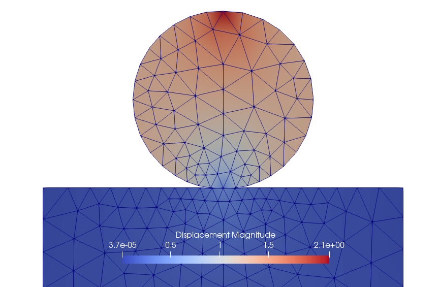For optimization loops, we want to programmatically find, for example, maximum contact pressure. We can, for example, get all the values in nodes:

lambda = contact("lambda", time)
normal = contact("normal", time)
p0 = 0.0
p0_acc = 3585.0
for (nid, n) in normal
    lan = dot(n, lambda[nid])
    println("$nid => $lan")
    global p0
    p0 = max(p0, lan)
end
p0 = round(p0, digits=2)
rtol = round(norm(p0-p0_acc)/max(p0,p0_acc)*100, digits=2)
println("Maximum contact pressure p0 = $p0, p0_acc = $p0_acc, rtol = $rtol %")

133 => 0.0
135 => 4056.017756303162
145 => 0.0
144 => 583.5173932223888
137 => 0.0
122 => 0.0
134 => 821.4109821942362
Maximum contact pressure p0 = 4056.02, p0_acc = 3585.0, rtol = 11.61 %

To get rough approximation where does the contact open, we can find the element from slave contact surface, where contact pressure is zero in the other node and something nonzero in the other node.

a_rad = 0.0
for element in contact_slave_elements
    la1, la2 = element("lambda", time)
    p1, p2 = norm(la1), norm(la2)
    a, b = isapprox(p1, 0.0), isapprox(p2, 0.0)
    if (a && !b) || (b && !a)
        X1, X2 = element("geometry", time)
        println("Contact opening element geometry: X1 = $X1, X2 = $X2")
        println("Contact opening element lambda: la1 = $la1, la2 = $la2")
        x11, y11 = X1
        x12, y12 = X2
        global a_rad
        a_rad = 1/2*abs(x11+x12)
        break
    end
end
println("Contact radius: $a_rad")

Contact opening element geometry: X1 = [13.658484560848699, 0.0], X2 = [6.566329883460562, 0.0]
Contact opening element lambda: la1 = [0.0, 0.0], la2 = [0.0, 583.5173932223888]
Contact radius: 10.11240722215463

This example briefly described some of the core features of JuliaFEM.

This page was generated using Literate.jl.